In this article we will discuss how to do image classification in Jupyter Notebook. We will create a classification using pictures from breast cells for predicting breast cancer disease.
First of all, let’s import the libraries to start the project.
Import libraries
import numpy as np # linear algebra
import pandas as pd # data processing, CSV file I/O (e.g. pd.read_csv)
import matplotlib.pyplot as plt
from sklearn.model_selection import train_test_split
from sklearn.metrics import accuracy_score
#import keras
#from keras.utils import to_categorical
from tensorflow.keras.utils import to_categorical
from keras.models import Sequential
from keras.layers import Dense, Dropout, Conv2D, MaxPool2D, Flatten
from keras.layers import Conv2D, MaxPooling2D
from keras.datasets import mnist
from keras.preprocessing import image
from keras.utils import np_utils
from tqdm import tqdm
Note: As you can see, there are a lot of libraries that we need to import, especially the keras one. The reason why we need a lot of libraries is because deep learning requires many processes from the input process to the output, which requires many layers in order to run properly.
After we imported the library, we need to import the dataset for this project. In this project, we will use the dataset from a collaboration between P&D Laboratory and Pathological Anatomy and Cytopathology, Parana, Brazil.
df = pd.read_csv("input/breakhis/Folds.csv")
df = df.sample(frac=1)
path = "input/breakhis/BreaKHis_v1/"
Dataframe from dataset
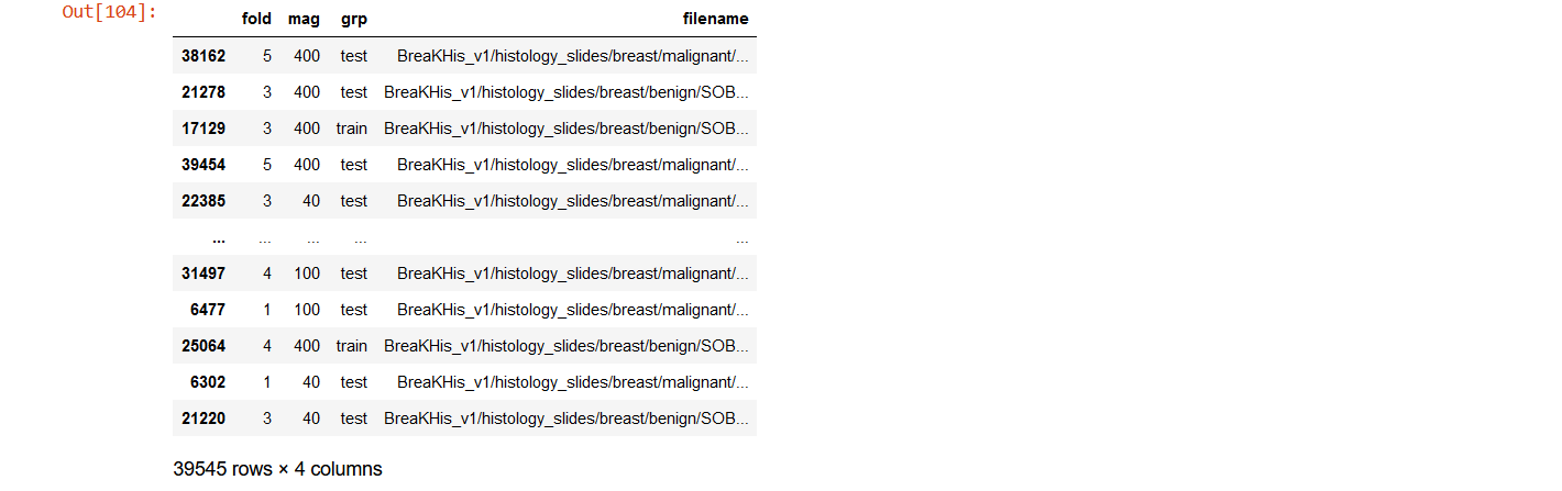
Next, we need to classify between the pictures to know which is benign and malignant cells.
Classify the image
train_image = []
y = []

for i in tqdm(range(df.shape[0])):
    img = image.load_img(path + df['filename'].iloc[i], target_size=(28,28,1), grayscale=False)
    img = image.img_to_array(img)
    img = img/255
    train_image.append(img)

    if (df['filename'].iloc[i].find('benign') != -1):
        y.append(0)
    else:
        y.append(1)
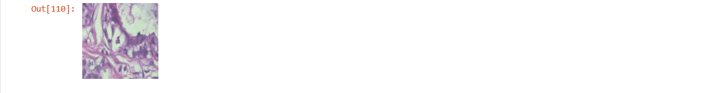
Here are some example pictures of benign and malignant cells.
Benign Cell

Malignant cell
After that, we need to split the data for data training and data validation.
Split the data
X = np.array(train_image)
y = np.array(y)

X_train, X_test, y_train, y_test = train_test_split(X, y, random_state=42, test_size=0.3)
X_test, X_val, y_test, y_val = train_test_split(X_test, y_test, random_state=42, test_size=0.3 , shuffle=True)

Y_train = np_utils.to_categorical(y_train, 2)
Y_test = np_utils.to_categorical(y_test, 2)
Y_val = np_utils.to_categorical(y_val, 2)

print(X_train.shape)
print(X_test.shape)
print(X_val.shape)
Then, we create the model for classification using CNN Algorithm
Create the model
model = Sequential()
#convlouton layer with the number of filters, filter size, strides steps, padding or no, activation type and the input shape.
model.add(Conv2D(30, kernel_size = (3,3), strides=(1,1), padding='valid', activation='relu', input_shape=(28,28,3)))
#pooling layer to reduce the volume of input image after convolution,
model.add(MaxPool2D(pool_size=(1,1)))
#flatten layer to flatten the output
model.add(Flatten())   # flatten output of conv
model.add(Dense(150, activation='relu'))  # hidden layer of 150 neuron
model.add(Dense(2, activation='softmax'))  # output layer
model.compile(loss='categorical_crossentropy', metrics=['accuracy'], optimizer='adam')

history = model.fit(X_train, Y_train, batch_size=10, epochs = 10, validation_data=(X_val, Y_val))
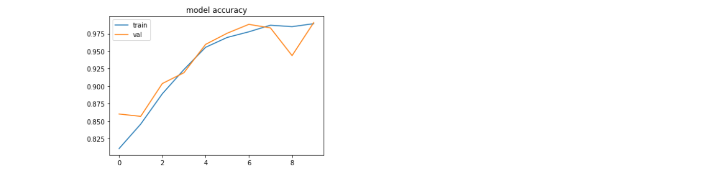
After all of that, we need to check the model accuracy and model loss, which is the way to know whether the model is good or not.
Here are the pictures of model accuracy and loss.
Model Accuracy
Model Loss

If you need more information regarding the model, you can add a few more codes to add more information. Here are the some code examples for adding information :
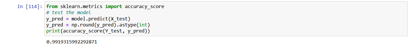
Check model accuracy using sklearn
from sklearn.metrics import accuracy_score
# test the model
y_pred = model.predict(X_test)
y_pred = np.round(y_pred).astype(int)
print(accuracy_score(Y_test, y_pred))
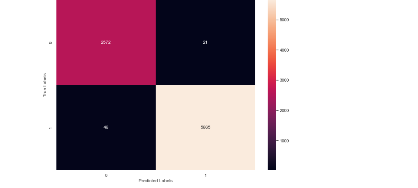
Create confusion matrix
import sklearn
from sklearn.metrics import confusion_matrix
cm=sklearn.metrics.confusion_matrix(Y_test.argmax(axis=1), y_pred.argmax(axis=1))
print(cm)

import seaborn as sns
import matplotlib.pyplot as plt
sns.set(rc={'figure.figsize':(11.7,8.27)})
sns.heatmap(cm, annot=True, fmt='.4g')
plt.xlabel('Predicted Labels')
plt.ylabel('True Labels')
plt.show()
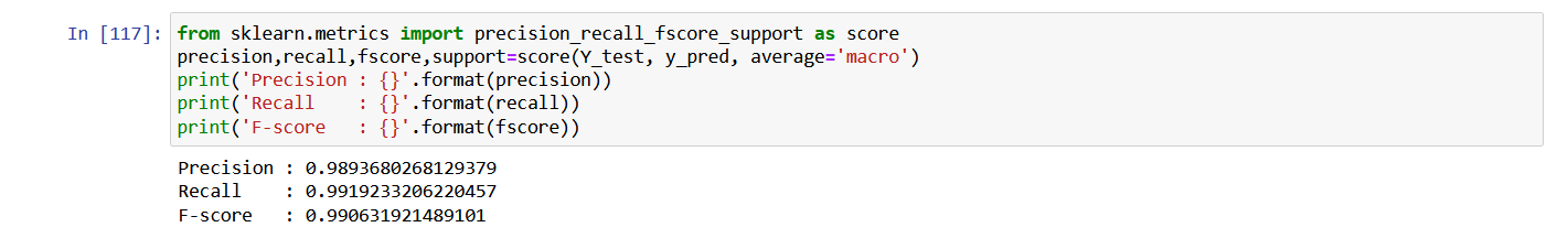
Check precision, recall, f1-score
from sklearn.metrics import precision_recall_fscore_support as score
precision,recall,fscore,support=score(Y_test, y_pred, average='macro')
print('Precision : {}'.format(precision))
print('Recall    : {}'.format(recall))
print('F-score   : {}'.format(fscore))
Dataset Link: Breakhis Dataset